Lecture IX - Data Visualization

Programming with Python

Dr. Tobias Vlćek

Kühne Logistics University Hamburg - Fall 2026

EP 9: The Pitch Deck

Charts are arguments

Friday, the boardroom. Picture it: the investor slides a pencil out of her jacket and sharpens it while you set up, the sound louder than it has any right to be.

Last week you handed her a table she could trust. She read exactly one row, looked up, and said the thing this whole session is about:

“Tables are homework. Charts are arguments.”

Your agent draws any chart in five seconds, so drawing is no longer the hard part. Today: which chart to draw, what it should say, and in which order you show the charts.

One download first

On a Mac? Open a terminal now and type:

git --version

A window offers to install the command line developer tools? Click Install and let it run while we talk. It’s a big download, and you need git before today’s lab.

On Windows, or a version number came back? Nothing to do yet.

Warm-up

Question 1

Three questions from Episode 8. Commit. Hands up before the reveal.

orders[orders["zone"] == "Nord"]

returns…

a) a True/False column
b) only the Nord rows
c) an error from comparing text

Answer 1

orders[orders["zone"] == "Nord"]
order_id zone items total_eur
0 101 Nord 2 18.5
2 103 Nord 3 24.0

b) only the Nord rows: the True/False column is what the inner expression orders["zone"] == "Nord" makes. Wrapped in orders[...], that mask keeps the rows where it’s True and drops the rest.

Question 2

orders.groupby("zone")["total_eur"].sum()

returns…

a) one row per order, with its zone
b) one total for all orders
c) one total per zone

Answer 2

orders.groupby("zone")["total_eur"].sum()
zone
Hafen     6.8
Nord     42.5
Sued     38.6
Name: total_eur, dtype: float64

c) one total per zone: groupby splits the orders by zone, .sum() adds up each group. Today this table sits behind every bar chart: the bars have to match it.

Question 3

orders["total_eur"].describe()

shows…

a) the first five rows of the column, like .head()
b) count / mean / std / min / quartiles / max
c) the column’s dtype, like .dtypes

Answer 3

orders["total_eur"].describe()
count     5.000000
mean     17.580000
std      10.688873
min       6.800000
25%       7.200000
50%      18.500000
75%      24.000000
max      31.400000
Name: total_eur, dtype: float64

b) count / mean / std / min / quartiles / max. One line, the column’s whole statistical fingerprint.

Ugly, bad, wrong

Your agent draws, you judge

Ask your agent for a bar chart of revenue per dish:
import matplotlib.pyplot as plt

dishes = ["Pad Thai", "Miso Ramen",
          "Bao Box", "Falafel Wrap"]
revenue = [420, 450, 330, 300]

plt.figure()      # a fresh canvas
plt.bar(dishes, revenue)
plt.ylabel("Revenue (EUR)")
plt.title("Revenue per dish")
plt.gca()         # show it

Bar chart of revenue per dish: Pad Thai 420, Miso Ramen 450, Bao Box 330, Falafel Wrap 300 euros, drawn in the default blue with the y-axis labelled Revenue (EUR).

Read the code, don’t memorize it. Your job: judge the picture. Here, the names already collide.

Ugly, bad, wrong

Problem charts get one of three verdicts (Wilke 2019, ch. 1):

  • Ugly: clear and correct, but unpleasant to look at
  • Bad: the numbers are right, but the picture is unclear, confusing, overloaded or deceiving
  • Wrong: the numbers in the picture are not the data

Fix wrong first, then bad. Ugly comes last: a correct, clear chart in default colors already does its job.

Predict: which chart is wrong?

Three drafts from Tobi’s agent. Exactly one is wrong:
Three charts of the same four dishes. Chart 1: bars labelled with shares of revenue of 32, 35, 25 and 23 percent. Chart 2: bars in magenta, green, yellow and cyan with thick black outlines and a heavy black grid. Chart 3: a pie with four slices of similar size and no numbers.

a) chart 1
b) chart 2
c) chart 3

Answer: chart 1 adds up to 115 %
Two bar charts of revenue shares per dish. Left, Tobi's agent: 32, 35, 25 and 23 percent, which add up to 115 percent. Right, the shares computed from the revenue: 28, 30, 22 and 20 percent, which add up to 100 percent.

a) chart 1: shares of one whole add up to 100 %, and these add up to 115 %. That’s wrong. Chart 2 is ugly: loud, but you can read every number. Chart 3 is bad for this question: correct, but nobody can tell which slice is biggest.

The title is a claim

A title states the point (Wilke 2019, ch. 22):

Describes the chart States the point
Revenue per dish Miso Ramen sells best: 450 euros
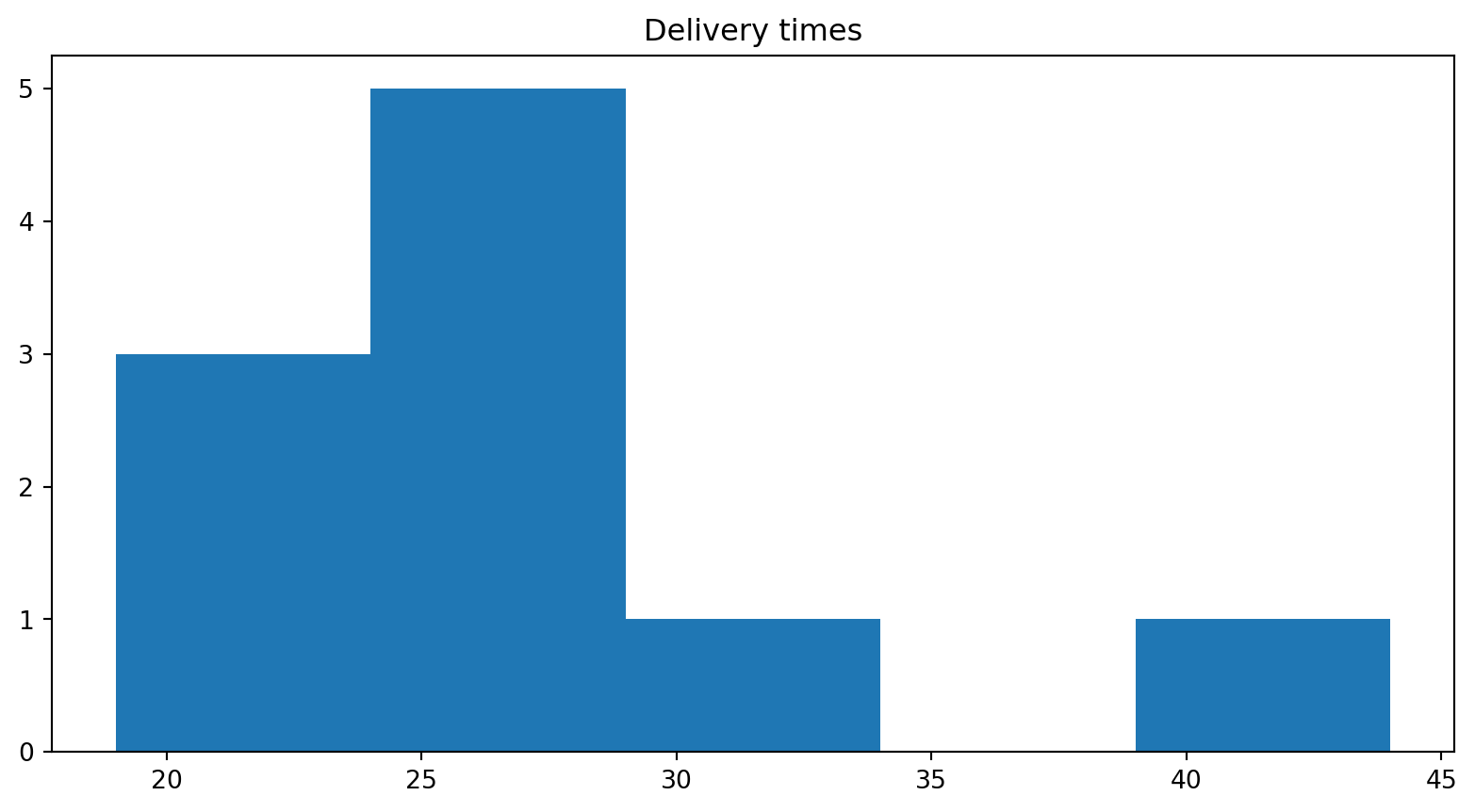
Delivery times Most deliveries take 20-30 minutes
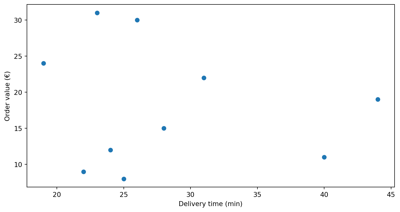
Order value vs. delivery time Big orders don’t take longer
  • Write the claim before you draw. If you can’t, the chart has no point yet.
  • Every axis names what it measures, with the unit: Revenue (EUR).

Your turn

Open the exercise

Scan the QR or type the link:

python.tobiasvlcek.com/notebooks/ex_09_a/

QR code linking to the online notebook for exercise 9a, the same address as the link above.

Any questions? Let me know!

Question first

MunchCorp’s one pie

The one chart in MunchCorp’s press release from Episode 8:
MunchCorp's pie chart of revenue per zone: four slices for Nord, Altstadt, Hafen and Sued, all close to a quarter of the circle, with no numbers on them.

Which zone brings MunchCorp the most?

a) Nord, top left
b) Hafen, bottom right
c) Altstadt, bottom left

Answer: Altstadt, by 1.4 points
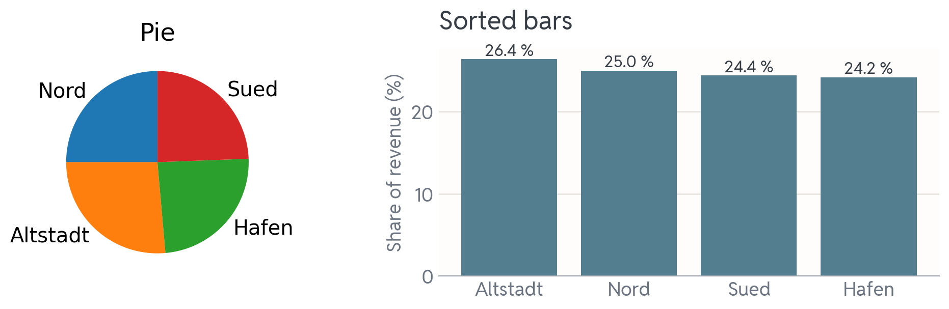
The same MunchCorp data twice. Left, the pie with four slices of nearly equal size. Right, sorted bars: Altstadt 26.4, Nord 25.0, Sued 24.4 and Hafen 24.2 percent, so the order is clear at a glance.

c) Altstadt: 26.4 % against Nord’s 25.0 %. The eye compares lengths well and areas badly. The sorted bars answer in a second; the pie starts an argument.

Match the chart to the question

The question The basic chart
How much per category? bar, sorted
How are values spread? histogram
What share of the whole? pie, for halves and quarters
Do two numbers move together? scatter
How does it change over time? line
Where, and how sure? map, error bars

A quick tour of each family (Wilke 2019, ch. 5):

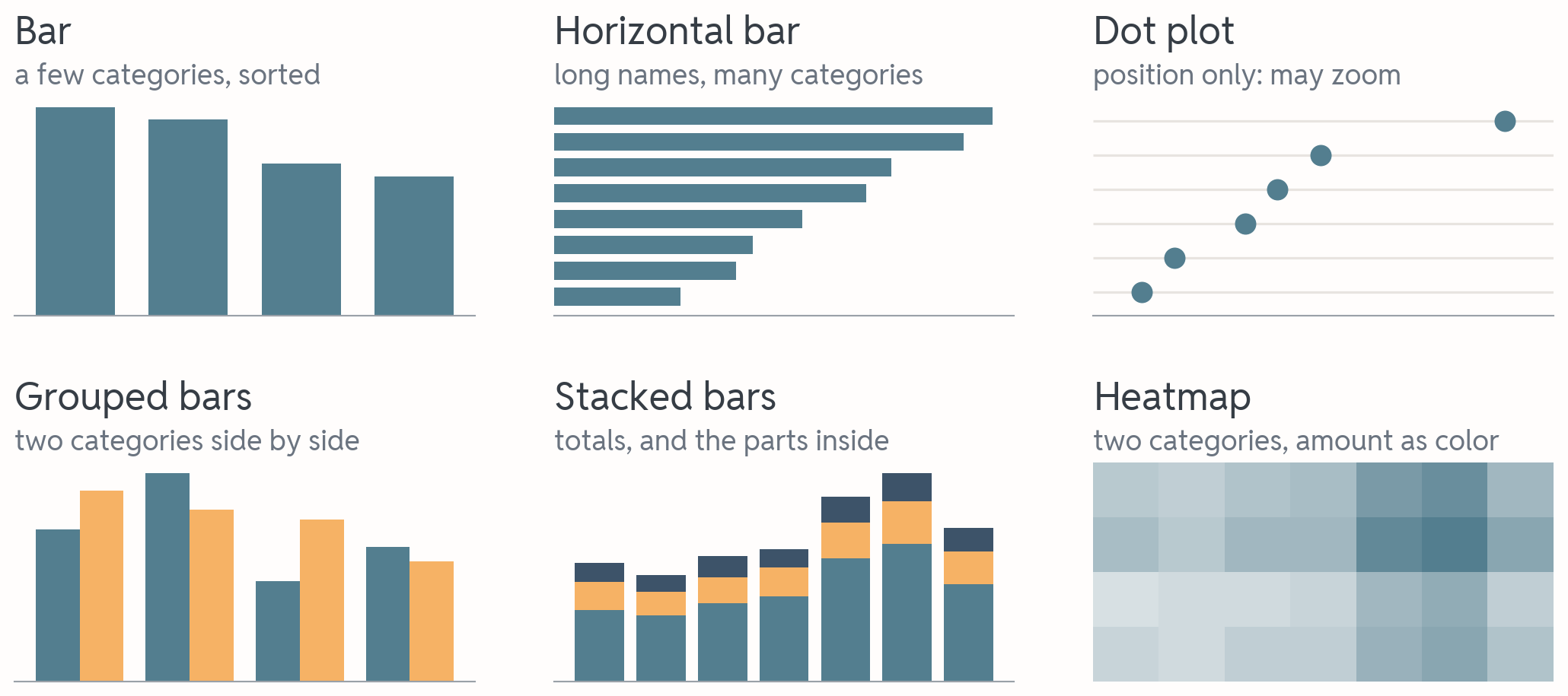
Amounts: how much?

Six small chart icons for amounts. Bar: four sorted bars. Horizontal bar: eight sorted bars lying down. Dot plot: six dots on a zoomed axis. Grouped bars: pairs of teal and sand bars. Stacked bars: seven bars split into three colored parts. Heatmap: a grid of squares, darker where the amount is larger.

Bars start at 0, a dot may zoom: the next block says why.

Distributions: how spread out?
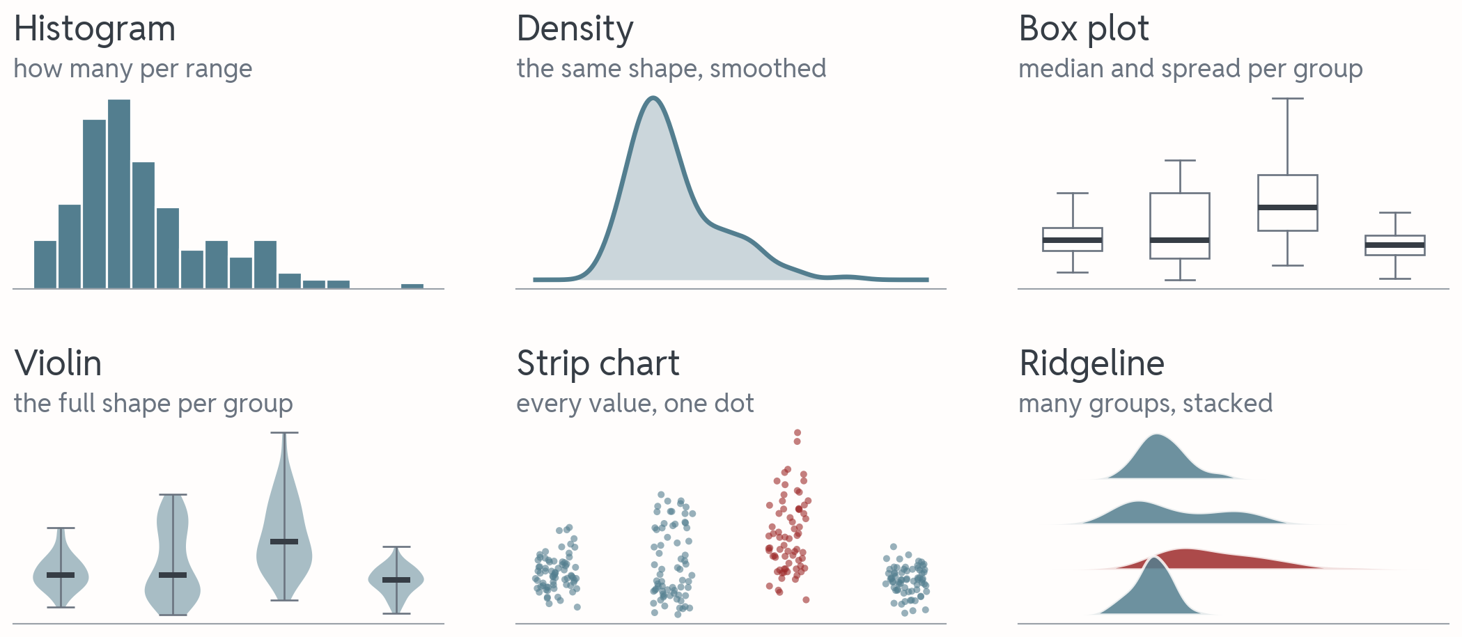
Six small chart icons for distributions of delivery times. Histogram: bars that pile up on the left with a long tail. Density: the same shape as a smooth filled curve. Box plot: four boxes with a dark red median line. Violin: four mirrored shapes, one with two bulges. Strip chart: four columns of dots, one in dark red. Ridgeline: four smooth curves stacked above each other.

Also in the directory: cumulative densities, q-q and sina plots.

Proportions: what share?
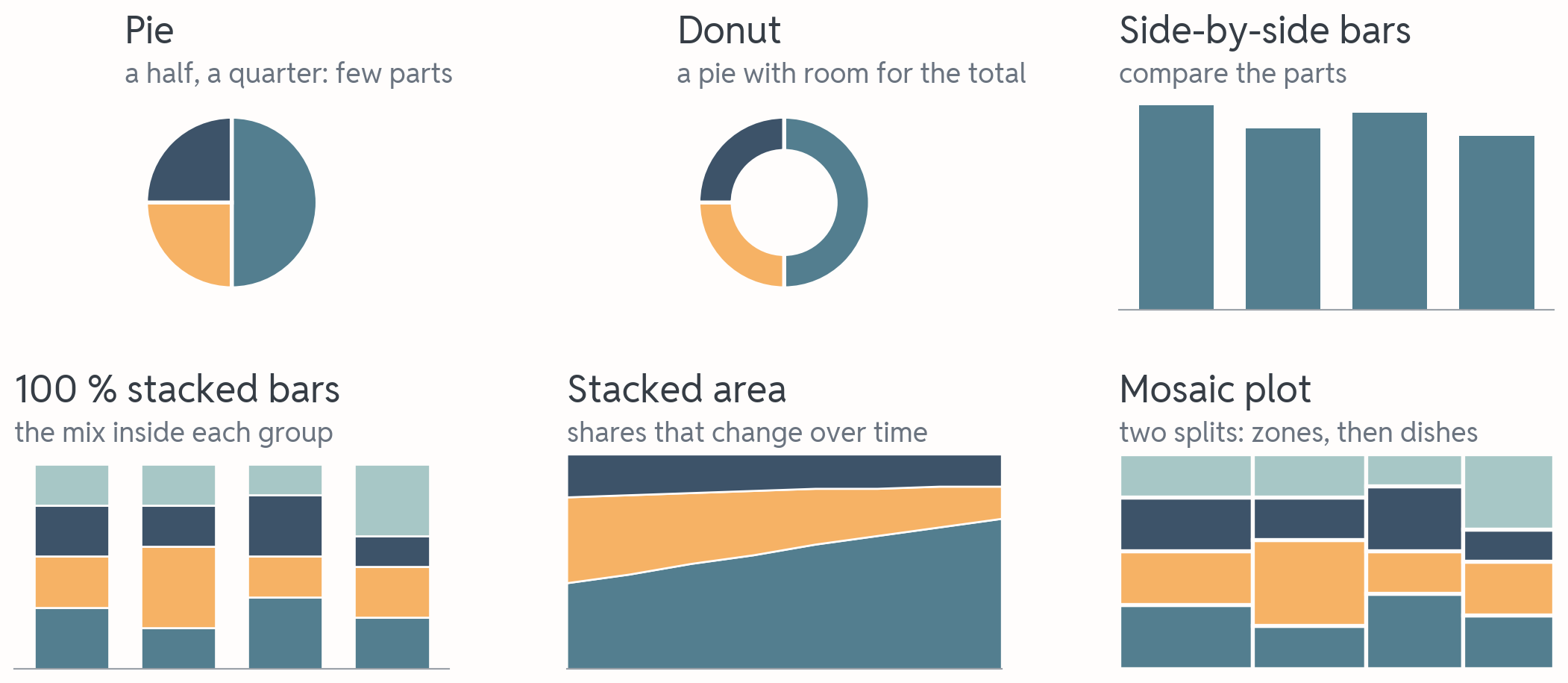
Six small chart icons for shares. Pie: a half and two quarters. Donut: the same as a ring. Side-by-side bars: four bars of nearly equal height. 100 percent stacked bars: four columns of equal height split into four colors. Stacked area: three colored bands, the bottom one growing. Mosaic plot: one rectangle split into columns by zone, each column split into colored blocks by dish.

Also in the directory: treemaps, parallel sets, nested pies.

Relationships: two numbers
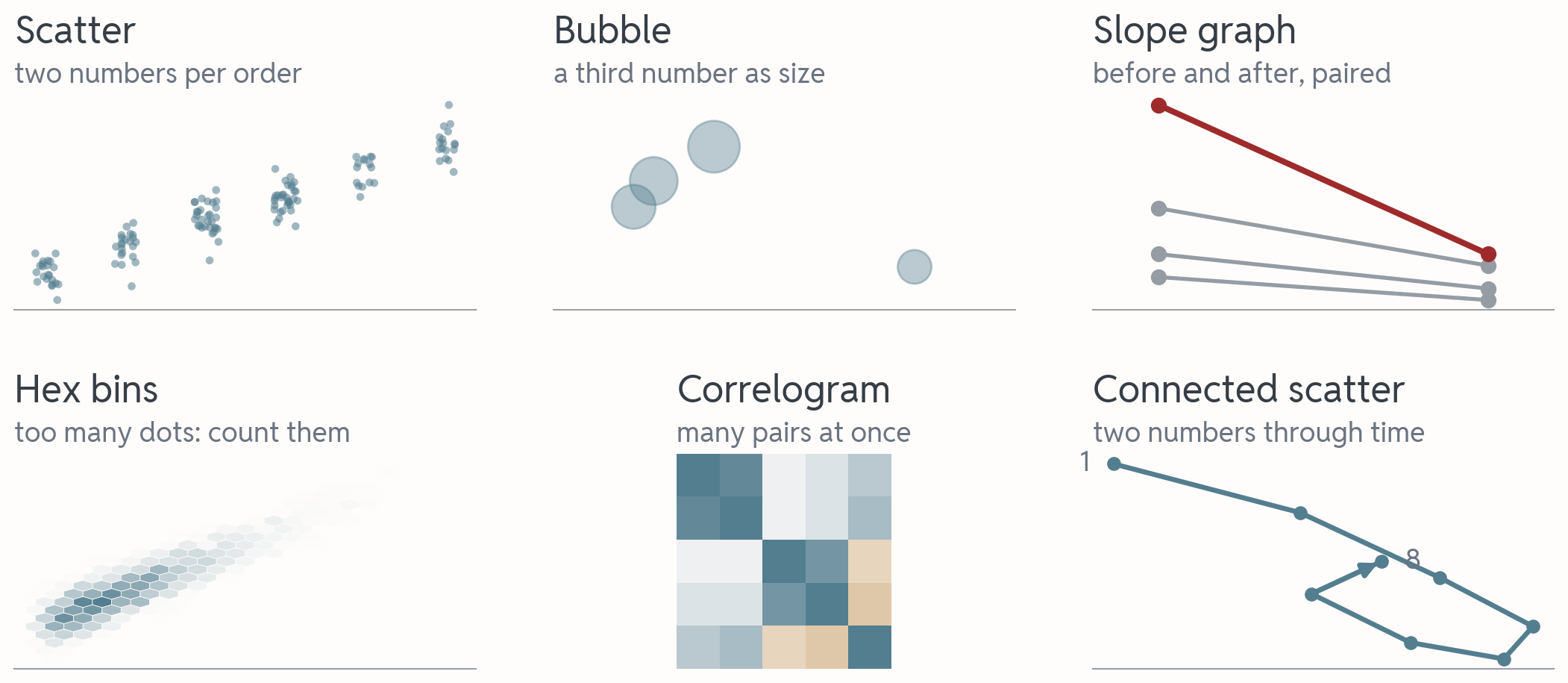
Six small chart icons for relationships. Scatter: a cloud of dots rising to the right. Bubble: four dots of different sizes. Slope graph: four lines from a left column to a right column, one dark red line falling steeply. Hex bins: a rising band of hexagons, darkest in the middle. Correlogram: a five by five grid of squares in teal and red shades. Connected scatter: dots joined in time order from week 1 to week 8, moving down to the right and then turning back, with an arrow on the last step.

A shapeless cloud is a finding too: it goes in the title like any claim.

Time series: change over time
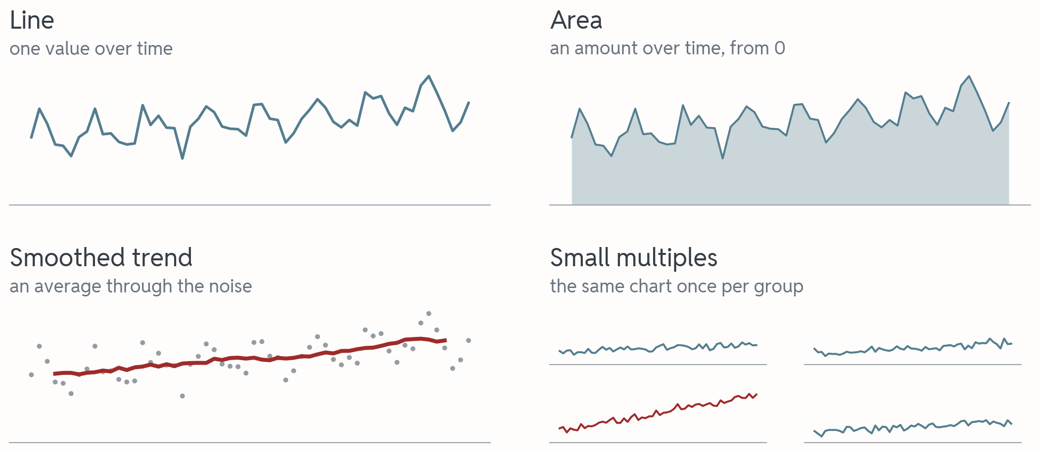
Four small chart icons for time series. Line: a rising line with a weekly ripple. Area: the same shape filled down to zero. Smoothed trend: faint dots with a dark red average line through them. Small multiples: four tiny line charts in a grid, one of them dark red and rising faster.

Many lines? One accent, the rest grey. More after the break.

Maps and uncertainty
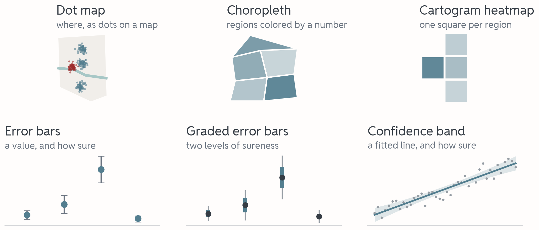
Six small chart icons. Dot map: clusters of dots inside a pale city outline with a river, one cluster dark red. Choropleth: five irregular regions shaded from light to dark teal. Cartogram heatmap: four equal squares in shades of teal. Error bars: four dots, each with a vertical bar for how sure the value is. Graded error bars: the same with a thick inner and a thin outer bar. Confidence band: dots with a fitted line inside a pale band.

Also in the directory: cartograms, eyes plots, quantile dots.

Predict: how many bars?

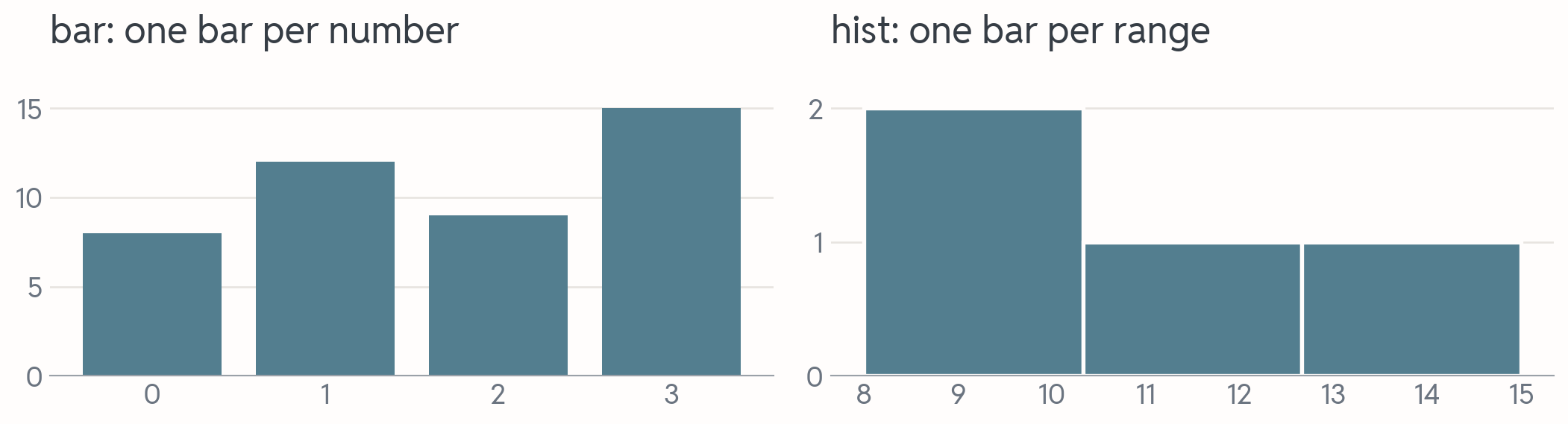
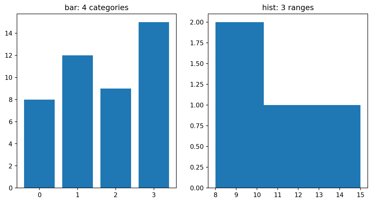
The same four numbers, two ways. On the left, a bar per number; on the right, a histogram:

values = [8, 12, 9, 15]
plt.bar(range(4), values)   # left
plt.hist(values, bins=3)    # right

The bar chart shows 4 bars. How many bars does the histogram show?

a) 4: one bar per number
b) 15: one bar per unit up to the max
c) 3: one bar per range

Answer: three ranges, three bars

Two panels from the same four numbers. Left, a bar chart with four bars of heights 8, 12, 9 and 15. Right, a histogram with three separate bars for three ranges between 8 and 15, of heights 2, 1 and 1: 8 and 9 share the first range.

c) 3: 8 and 9 share the first range, so that bar is 2 tall. A bar chart shows one bar per category, as tall as its value. A histogram shows one bar per range, as tall as the number of values in it.

Your turn

Open the exercise

Scan the QR or type the link:

python.tobiasvlcek.com/notebooks/ex_09_b/

QR code linking to the online notebook for exercise 9b, the same address as the link above.

Any questions? Let me know!

Proportional ink

Predict: how many times more?

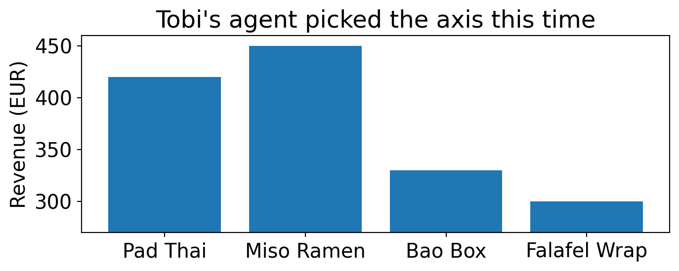
Bar chart of revenue per dish with the y-axis running from 270 to 460 euros: Pad Thai 420, Miso Ramen 450, Bao Box 330, Falafel Wrap 300. The Miso Ramen bar looks about six times as tall as the Falafel Wrap bar.

Miso Ramen vs. Falafel Wrap: how many times as much?

a) about 1.5 times
b) about 3 times
c) about 6 times

Answer: 1.5 times, drawn as 6
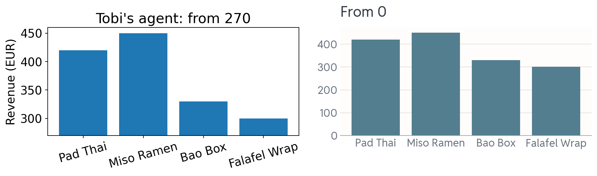
The dish revenue twice. Left, Tobi's agent with the y-axis from 270: the Miso Ramen bar is six times as tall as the Falafel Wrap bar. Right, the same bars from 0: Miso Ramen 450 against Falafel Wrap 300, one and a half times as tall.

a) about 1.5 times: 450 against 300. Cut at 270, the bars keep 180 and 30 of their length, so the picture says 6 times. That’s bad: the numbers are right, the picture misleads. The rule behind it is proportional ink: the ink for a value has to grow with the value (Wilke 2019, ch. 17).

Predict: the AI’s one extra line

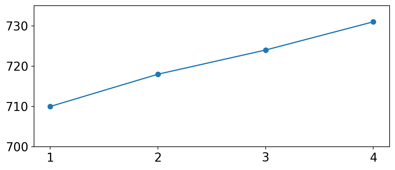
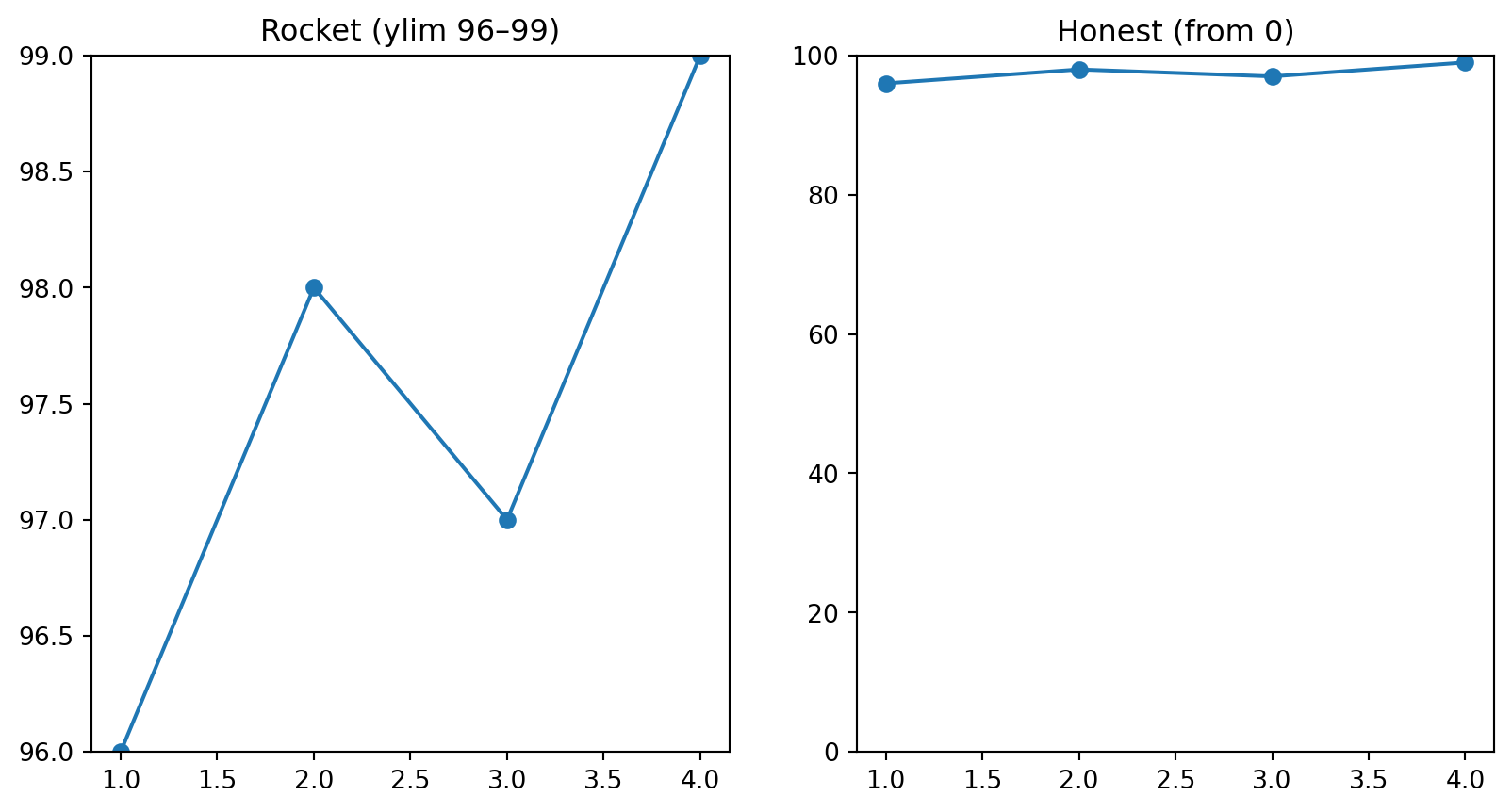
Revenue [710, 718, 724, 731], up 3 % over four weeks. Tobi’s AI drafts the chart and adds one line:

plt.plot([1, 2, 3, 4], [710, 718, 724, 731])
plt.ylim(700, 735)

What does the room see?

a) a flat line: 3 % stays 3 % on any axis
b) an error: ylim has to include zero on a line chart
c) a line rising across most of the chart

Answer: a climb across the chart

Line through 710, 718, 724 and 731 on a y-axis that runs only from 700 to 735. The line climbs 60 percent of the chart height, so 3 percent of growth looks like a steep rise.

c) a line rising across most of the chart: the axis spans 35 units and the line rises 21 of them, 60 % of the picture for 3 % of growth. Python raises no error.

Bars from zero, dots may zoom

  • A bar shows its number by its length: cut the axis and the comparison breaks. Bars always start at 0.
  • A dot shows its number by position only, so a dot plot may zoom (Wilke 2019, ch. 17).
  • A line sits in between: zooming blows a small change up. Plot the change from 0, or put its size in the title: “+3 % in four weeks”.

The investor reads the axis before the line, and then the title, to see if the two agree.

Your turn

Open the exercise

Scan the QR or type the link:

python.tobiasvlcek.com/notebooks/ex_09_c/

QR code linking to the online notebook for exercise 9c, the same address as the link above.

Any questions? Let me know!

A five-minute pause after this one, then three charts, made over step by step.

Make one point

Makeover 1: who is fastest?

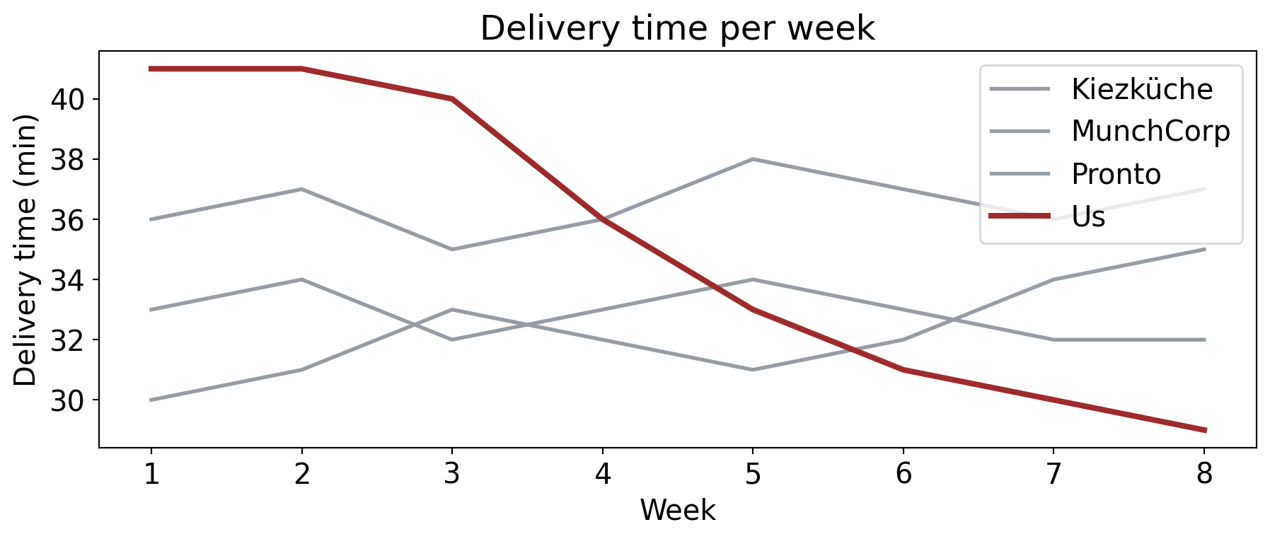
“Are you faster than the rivals?” First: who was fastest in week 1?
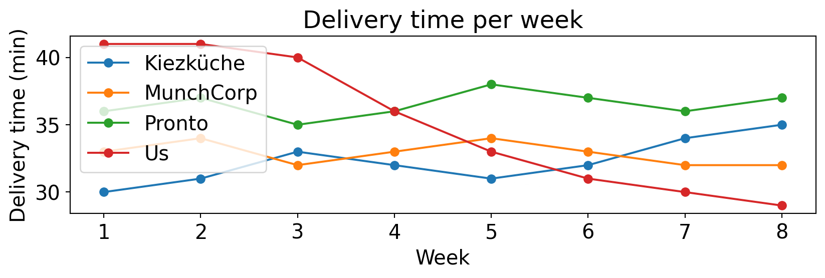
Default line chart of delivery time per week for eight weeks: four lines in blue, orange, green and red with dots, and a legend in alphabetical order, Kiezküche, MunchCorp, Pronto, Us. The lines cross each other several times.

a) MunchCorp
b) Kiezküche
c) Pronto

Answer: Kiezküche, the slow way

b) Kiezküche: 30 minutes in week 1. An easy number, found the slow way: you matched four colors to a legend sorted from A to Z. And her real question, whether we got faster, is buried even deeper.

The data is fine. The chart is bad: the point is in there, buried. Four changes dig it out, one at a time, and none of them touches the numbers.

Lines, step 1: one accent color

The same chart, with our line in dark red and thicker, and the three rival lines in light grey. The legend is still there.

Take the color out of everything except the point (Wilke 2019, ch. 4). One color= per line, and the eye knows where to go.

Lines, step 2: labels, no legend
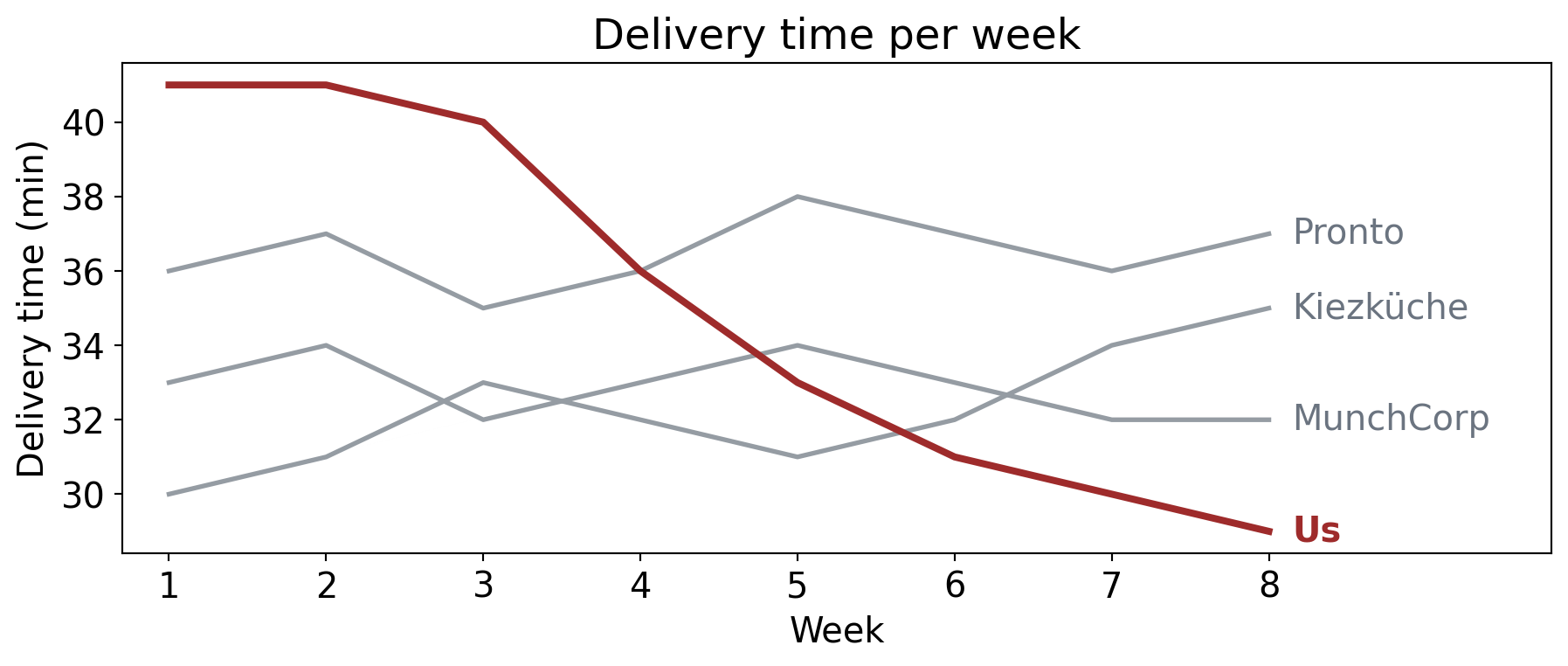
The same chart without a legend: each line now carries its name at its right end, Us in dark red at 29 minutes, the rivals in grey at 32, 35 and 37 minutes.

Names at the lines replace the legend, and they work for the 8 % of men who can’t tell red from green (Wilke 2019, ch. 19).

Lines, step 3: the title says it
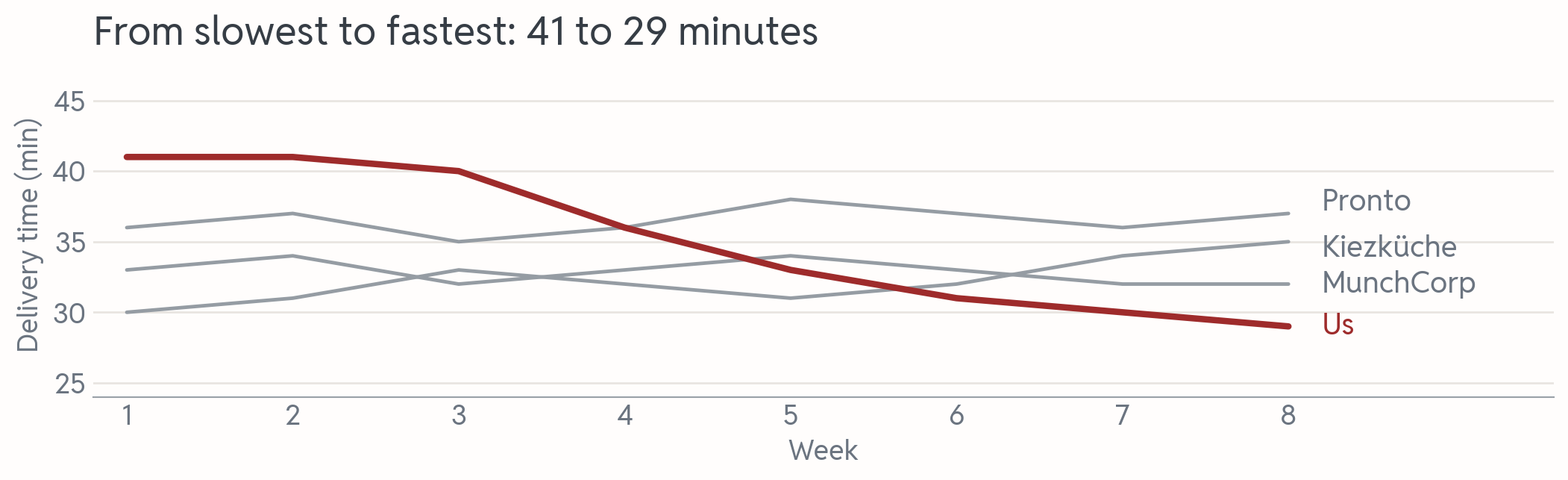
The chart in the house style: the title reads From slowest to fastest in eight weeks. Our dark red line falls from 41 to 29 minutes, the grey rival lines stay between 30 and 38, every line carries its name, and the frame and tick marks are gone.

The title states the claim; frame and tick marks are gone. Same numbers, and every change was a decision.

Lines, step 4: add the context
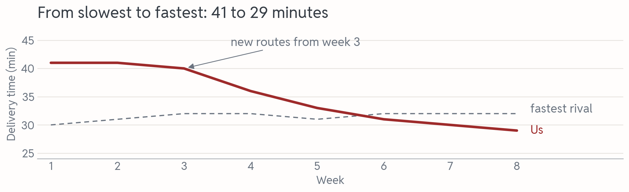
The same chart with context: the three grey rival lines are replaced by one dashed line labelled fastest rival, at 30 to 32 minutes, and a note with an arrow marks new routes from week 3, where our dark red line starts to fall. Our line drops below the dashed line in week 6.

The rivals only matter as a yardstick: one dashed line for the fastest rival replaces three, and one note marks week 3. Now the chart tells a story.

Lines, step 5: one too many
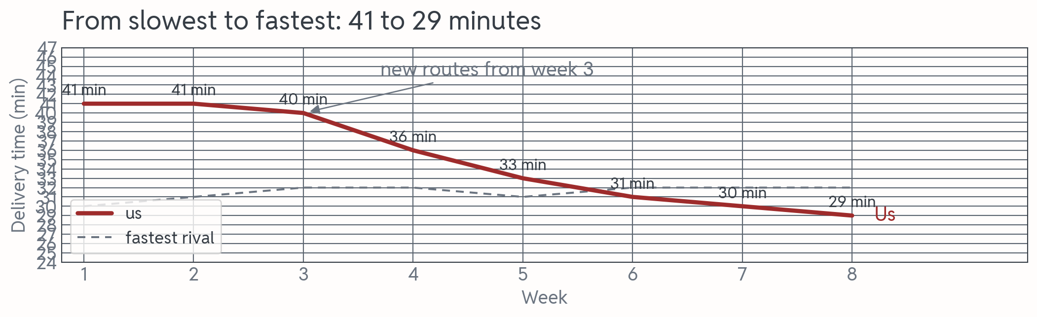
The step-4 chart buried under extras: a dark grid every minute, a full black frame, a boxed legend, and the number of minutes printed next to every point of our line. The point is still there but hard to find.

Every number, line and box here is true, and none of them helps: the point drowns. Balance data and context (Wilke 2019, ch. 23): stop at step 4.

Makeover 2: what misleads?
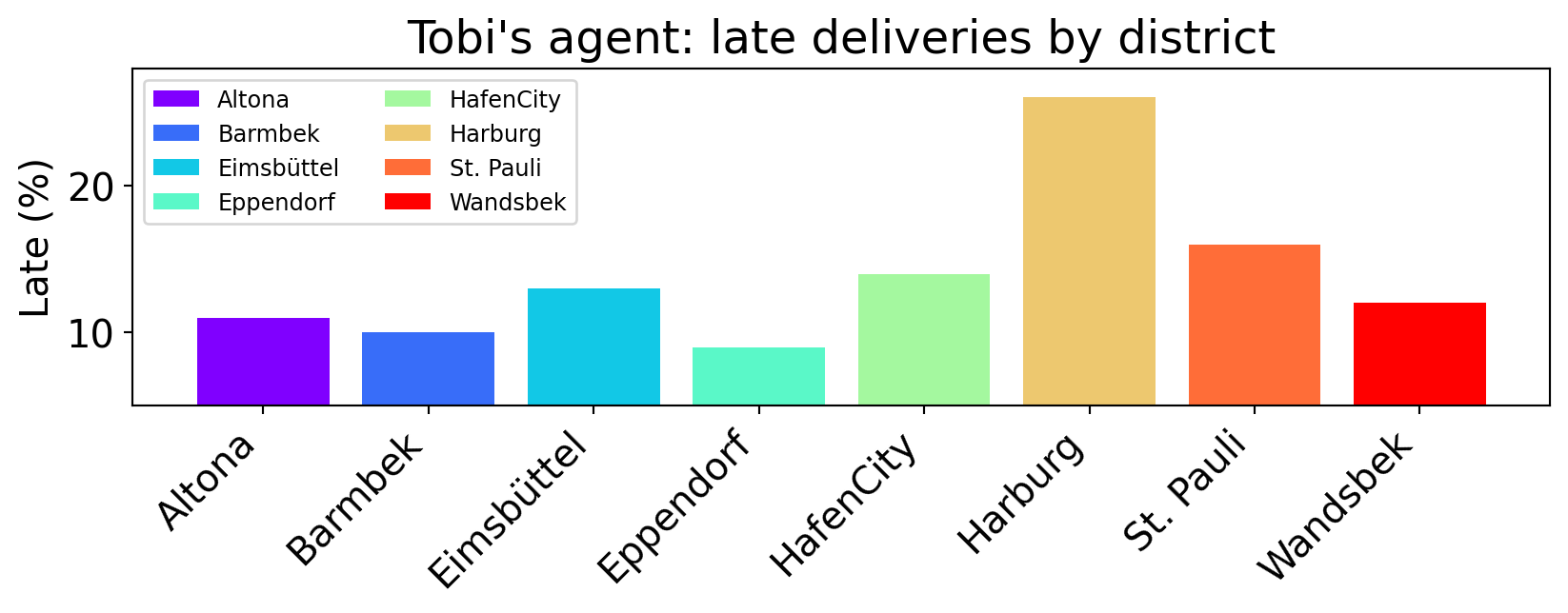
Tobi's agent's bar chart of late deliveries in eight districts in alphabetical order: every bar a different rainbow color, a legend that repeats the district names, names tilted at 45 degrees, and a y-axis that starts at 5 percent. Harburg's bar is by far the tallest.

Which problem makes the investor believe something false?

a) the loud colors
b) the axis from 5 %
c) the tilted names

Bars, step 1: from zero
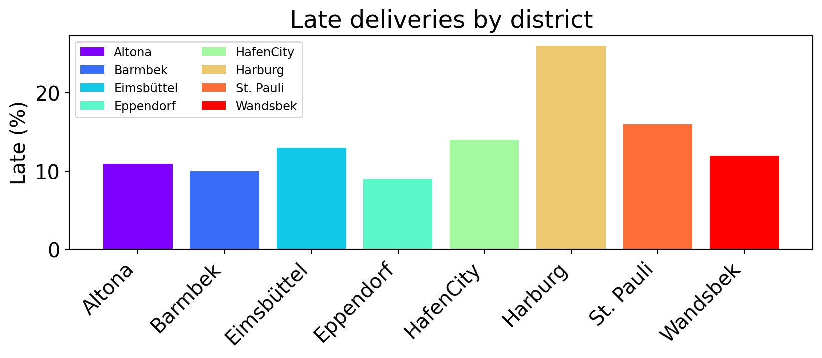
The same rainbow bar chart with the y-axis from 0. Harburg's bar at 26 percent is now about three times as tall as Eppendorf's at 9 percent.

b) the axis. Cut at 5 %, Harburg looked five times as late as Eppendorf; from 0 it is three times. The colors and the tilt only make the chart harder to read. Fix what misleads first.

Bars, step 2: sorted, lying down
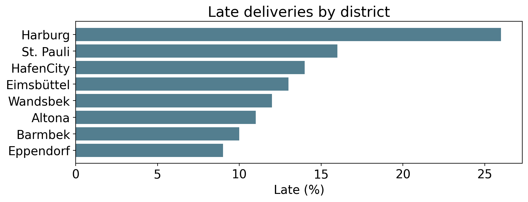
Horizontal bars in one color, sorted from Harburg at the top with 26 percent down to Eppendorf with 9 percent. The names read without tilting and the legend is gone.

Sorted, the ranking reads from top to bottom. Lying down, the names need no tilt. The colors meant nothing, so one color is enough, and the legend goes with them.

Bars, step 3: one point
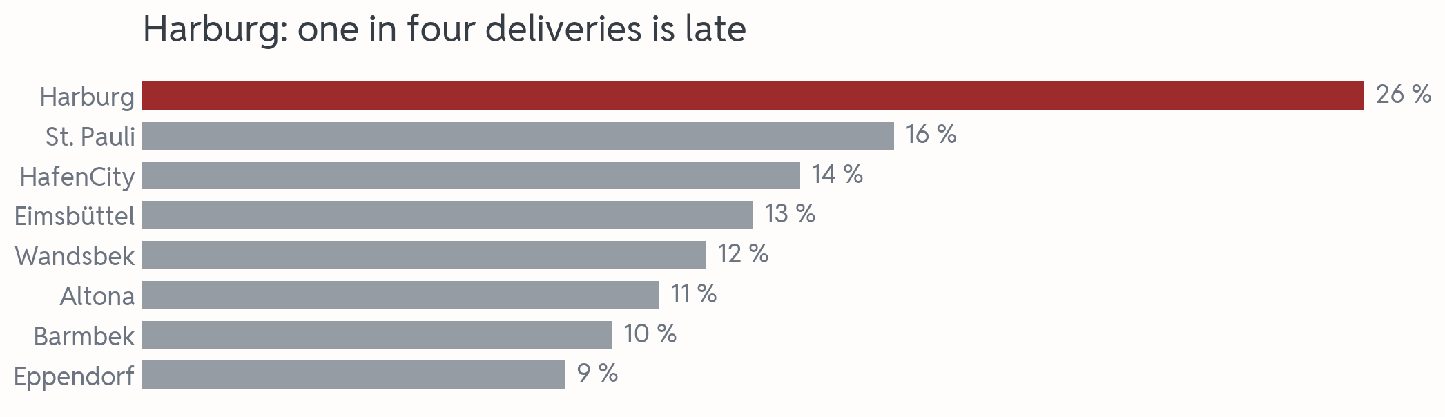
The finished chart: horizontal grey bars sorted by size, Harburg's bar on top in dark red, each bar with its percentage written at its end, no x-axis, and the title Harburg: one in four deliveries is late.

One accent for the point, the numbers on the bars instead of an axis, the claim on top. Step 1 fixed what misleads, step 2 what confuses, step 3 makes the point.

Makeover 3: who is late?
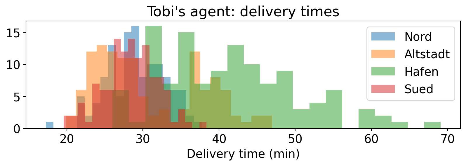
Four overlapping histograms of delivery times in the default blue, orange, green and red, half transparent, with a legend for Nord, Altstadt, Hafen and Sued. The colors mix where the bars overlap, and a green tail reaches beyond 60 minutes.

We promise 35 minutes. Which zone breaks it most often?

a) Altstadt, orange
b) Hafen, green
c) Nord, blue

Spread, step 1: one panel each
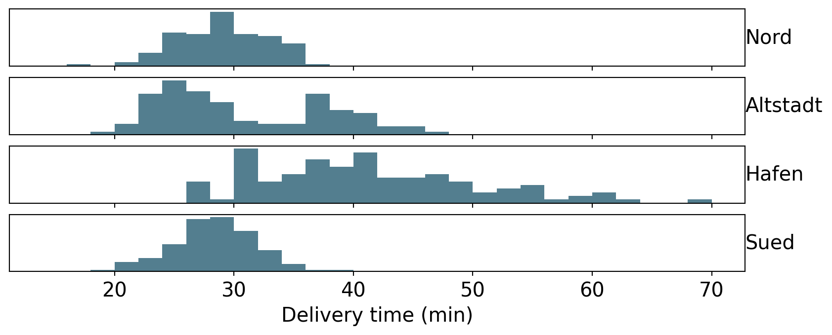
The same delivery times as four small histograms stacked above each other on one shared minutes axis. Nord and Sued sit around 28 minutes, Altstadt has two humps at about 26 and 39 minutes, and Hafen's bars spread far to the right.

b) Hafen: three of four deliveries take longer than 35 minutes. One panel per zone shows it, and shows what the overlap hid: Altstadt has two humps, a fast group and a slow one.

Spread, step 2: boxes and dots
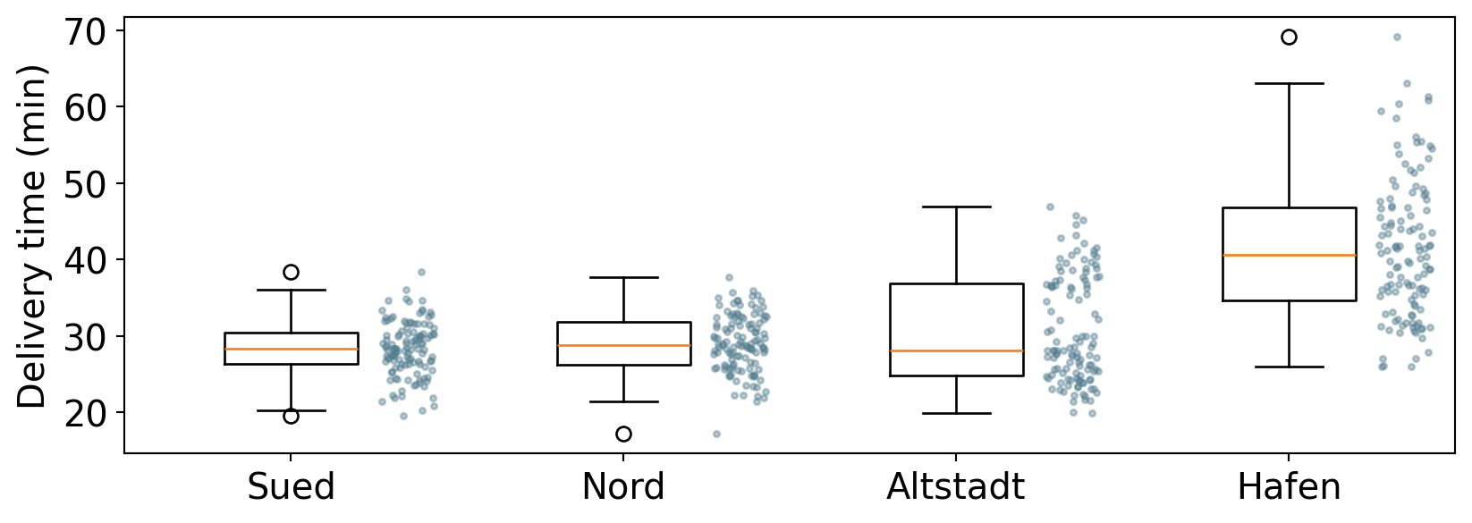
One chart with a box plot per zone, sorted from the most punctual zone, Sued, to Hafen, and every single delivery as a dot next to its box. Hafen's box sits highest, and Altstadt's dots form two clusters.

One chart instead of four: a box per zone for median and spread, every delivery as a dot beside it, from the most punctual zone to the least.

Spread, step 3: draw the promise
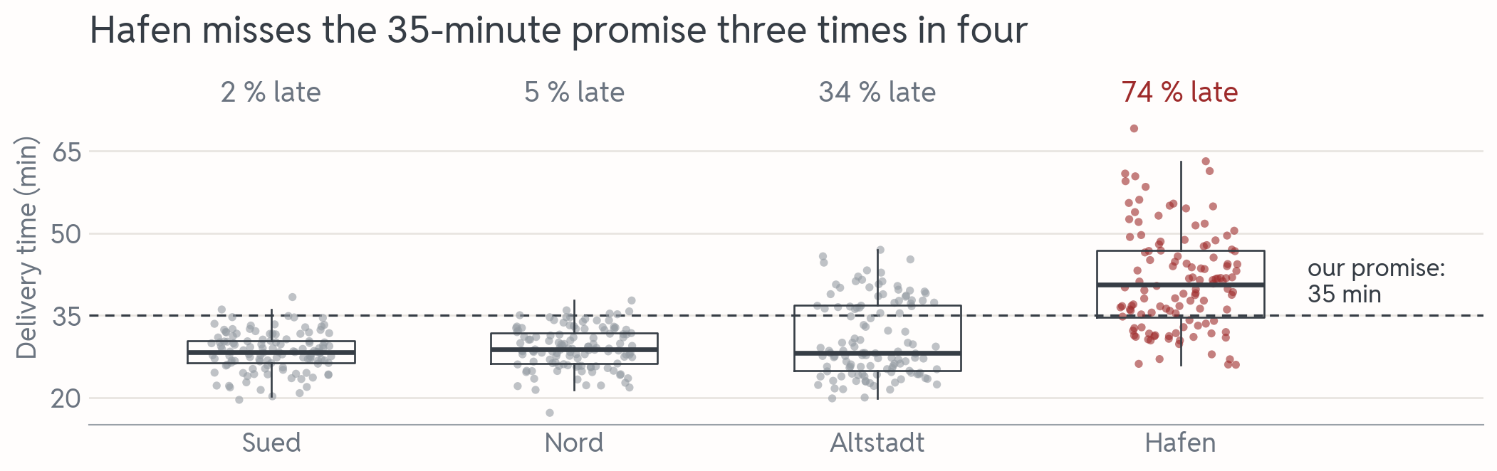
The finished chart: dots for every delivery per zone, grey for Sued, Nord and Altstadt and dark red for Hafen, a thin box over each zone, and a dashed line at 35 minutes labelled our promise. Most of Hafen's dots lie above the line. The title reads Hafen misses the 35-minute promise three times in four.

A reference line turns the chart into a test: every dot above it is a broken promise. The share on top and the title give the number.

Your turn

Open the exercise

Scan the QR or type the link:

python.tobiasvlcek.com/notebooks/ex_09_d/

QR code linking to the online notebook for exercise 9d, the same address as the link above.

Any questions? Let me know!

Charts to a story

A deck is a story

A story is facts in a specific order that create a reaction (Wilke 2019, ch. 29). A pitch in four steps:

  1. Opening: where we stand
  2. Challenge: the problem
  3. Action: what we did about it
  4. Resolution: the result, and what we ask for

Each step is one slide with one point, a figure for the generals: the room gets it in seconds.

Predict: Tobi’s four slides

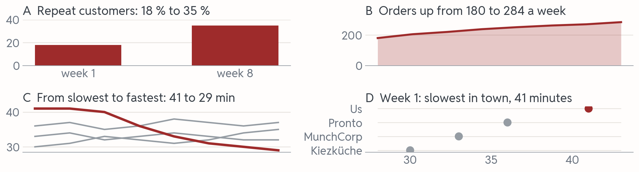
Four small slides with claim titles, each a different kind of chart. A: Repeat customers 18 percent to 35 percent, two dark red bars for week 1 and week 8. B: Orders up from 180 to 284 a week, a dark red area rising over eight weeks. C: From slowest to fastest, 41 to 29 minutes, our dark red line falling below three grey rival lines. D: Week 1, slowest in town, 41 minutes, a dot plot with our dot in dark red furthest right.

Opening, challenge, action, resolution: in which order?

a) B, D, C, A
b) A, B, D, C
c) B, C, D, A

Answer: B, D, C, A

The same four slides in story order: B, a rising dark red area of orders; D, the dot plot with us slowest; C, our line falling below the rivals; A, two bars for repeat customers rising from 18 to 35 percent.

a) B, D, C, A: a growing business (B), the slowest in town (D), new routes and a line that falls below every rival (C), customers who come back (A). Then the ask: one more rider keeps it that way.

Option b) leads with the result, an arc that works too, in a newspaper. In a pitch, the problem first makes the result count.

Two rules for the whole deck

  • Build up. Show our line alone before you add the rivals. A complex chart lands once the room has seen its simple version.
  • Keep colors fixed. Our line is dark red on every slide. Paint us blue on slide 3 and the room reads someone else’s line as yours.

Consistent, not repetitive: same colors and same fonts across the deck, but each slide a different kind of chart, so the room notices that something new is coming.

AI as your chart assistant

  1. Describe data and point: “Revenue per zone from orders (zone, total_eur), sorted bars, top zone dark red, rest grey, a title that names the leader.”
  2. Let it draft.
  3. Verify before you believe the picture:
    • the columns exist · the bars match your own groupby
    • bars from 0 · the chart type fits · the title says no more than the picture

AI drafts. You decide what goes on the slide.

Three ways AI charts mislead

  • Invented column names. It writes orders["revenue"], but your column is total_eur: the same confident nonsense you caught in Episode 8.
  • Defaults nobody chose. Bars in alphabetical order, one color per category, a legend, an axis cut to fit the data. Each one is a decision the agent made silently.
  • Your words as the title. Ask for a chart “showing that sales are growing” and that’s the title you get, whatever the line does.

For all three: check the numbers, the axis and the title before a chart goes on a slide.

Beyond matplotlib

Library What it adds
seaborn box, violin and histogram per group, in one line
plotly charts you can hover over and zoom into
folium street maps in the browser
streamlit a script becomes a web page with sliders
networkx networks of nodes and links

Next week’s project ideas use all five. Your agent writes the code; the checks from today stay the same.

Wrap-up

Three things to remember

  1. Judge every chart. Wrong first (shares that add up to 115 %), then bad (the pie), ugly last. Bars start at 0; a zoomed line needs a title with the real size.
  2. The question picks the chart, the title states the claim. Amounts → bar, spread → histogram, two numbers → scatter, time → line.
  3. One point per chart, one story per deck. One accent color, names on the lines, and the slides in an order that ends in your ask.

Season finale next: git and the project kickoff. Your laptop gets git now, before the lab.

Git before the lab

Why git, why today

Next session opens with Checkpoint 5, and then your project moves to GitHub. An installer that fights you then eats the project kickoff.

So we set up git now, together. Once your setup passes the check, open the lab; I come round and look at every laptop before you leave.

Step 1: git and gh

In Zed’s terminal (Ctrl+`), steps 1 and 2 of the one-time setup on the Git Basics page:

  • git: on a Mac git --version, on Windows winget install Git.Git
  • gh, the GitHub CLI: on Windows winget install GitHub.cli, on a Mac the installer linked on the page
  • Then quit and reopen Zed: its terminal only finds new programs after a restart

git --version and gh --version both print a version number? Step 1 is done.

Step 2: log in, say who you are

gh auth login
gh auth setup-git
git config --global user.name "Your Name"
git config --global user.email "you@example.com"
git config --global pull.rebase false
  • Login: GitHub.com, HTTPS, Yes to Authenticate Git, browser, one-time code
  • setup-git lets git use that login; it prints nothing
  • E-mail: the one of your GitHub account, it goes on every commit
  • pull.rebase false: a pull combines your partners’ work with yours

The check before the lab

git --version
gh auth status
git config --global user.email
  • a version number
  • Logged in to github.com account with your username, and Git operations protocol: https
  • the e-mail of your GitHub account

Open the lab as soon as all three print. I come round and check.

Stuck? Raise your hand early. Keep your phone at hand: GitHub may ask for a two-factor code, and a password you forgot since Session I is reset in two minutes. Only an iPad? Your GitHub codespace has git and gh built in: run the check in its terminal.

To the Lab

A chart in a script

The lab is a script, and a script has no cell that could show a chart. So every chart goes into a picture file:

plt.figure()                 # OPEN: a fresh canvas, as before
plt.plot(days, revenue)
plt.xlabel("Day")
plt.ylabel("Revenue (EUR)")
plt.title("Day 4 brings the most revenue")
daily_chart = plt.gca()      # KEEP: the chart, for the lab's checks
plt.savefig("daily.png")     # SAVE: the picture, into python-labs
plt.close()                  # CLOSE: the canvas

plt.close() puts the finished canvas away; the lab checks that none is left open. To look at the picture, click daily.png in Zed’s project panel, the file list on the left.

After the check: the lab

  • lab_09_pitch.py from Episode 9: The Pitch Deck into python-labs
  • Six charts, and you pick each kind. The investor gets four of them: you choose which, and in which order
  • Two things in Tobi’s deck are wrong, and no task says so: one in his numbers, one in his claims

Show me pitch_deck.png and the last block for feedback. Then practise the Checkpoint 5 hand-in once: open ex_09_d, Cmd/Ctrl+S, menu → Download → Download Python code.

Literature

Books to start with

Downey, Allen B. 2024. Think Python: How to Think Like a Computer Scientist. Third edition. O’Reilly. https://greenteapress.com/wp/think-python-3rd-edition/.
Wilke, C. 2019. Fundamentals of Data Visualization: A Primer on Making Informative and Compelling Figures. First edition. O’Reilly Media. https://clauswilke.com/dataviz/.

Both are free online. For this session, start with chapters 1, 17 and 29 of Wilke (2019).

Building charts with AI? Revisit the AI Tools page: describe-then-verify is the whole workflow. Matplotlib’s own pyplot tutorial is a friendly next step.

For more, see the literature list of this course.